
Price elasticity of supply (PES) is defined as a measure of the responsiveness of the quantity supplied of a good or service when there is a change in its price. It is calculated as PES = (% change in Qs) ÷ (% change in P). Supply is price elastic when PES > 1: a change in price causes a more than proportionate change in quantity supplied. Supply is price inelastic when PES < 1: a change in price causes a less than proportionate change in quantity supplied. The determinants of PES are the factors that decide how easily firms can change the quantity they supply when the price changes, and therefore whether supply is elastic or inelastic.
Figure 1 shows two diagrams, the left showing relatively elastic supply and the right showing relatively inelastic supply.
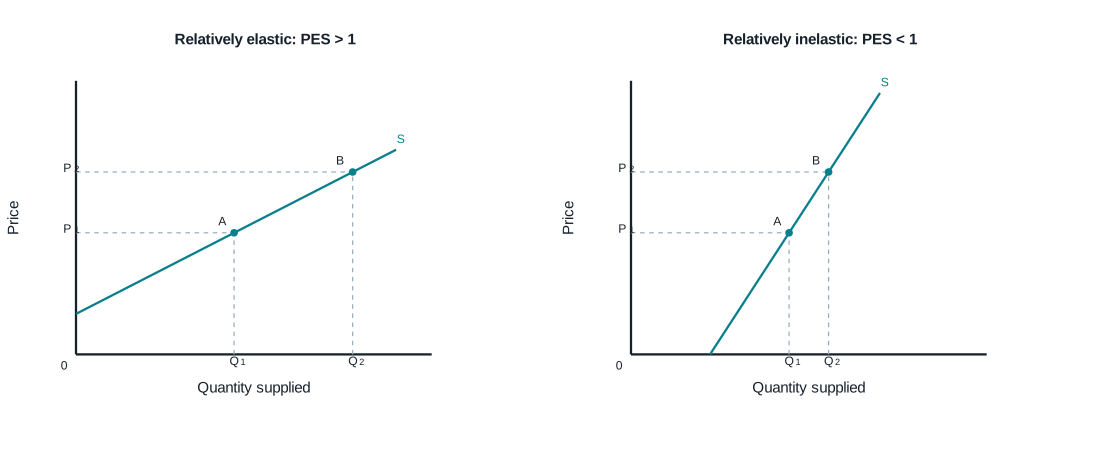
In the left panel of Figure 1, as price increases from P1 to P2, quantity supplied increases by a more than proportionate amount from Q1 to Q2. The percentage rise in quantity supplied is greater than the percentage rise in price, so supply is price elastic (PES > 1). In the right panel. as price increases from P1 to P2, quantity supplied increases by a less than proportionate amount. The percentage rise in quantity supplied is smaller than the percentage rise in price, so supply is price inelastic (PES < 1).
Two important factors affecting PES are the length of time firms have to respond to a price change and the amount of spare (unused) capacity firms have. Both affect how quickly and easily firms can increase or decrease their output when the price of their good changes.
Length of time: The longer the period of time firms have to adjust their inputs in response to a price change, the more elastic supply is. Over a very short time, firms may be unable to change their inputs at all, so they cannot change the quantity they supply. For example, when a fishing boat returns from a trip, it has only a fixed amount of fish to sell. Even if the price of fish rises, quantity supplied cannot respond, so supply is perfectly inelastic (PES = 0). This would be represented by S1 in figure 2. In figure 2, S₁ is vertical at Q₁ (the very short run). S₂ is relatively steep (the short run). S₃ is relatively flat (the long run).
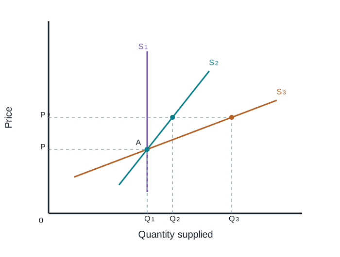
As more time passes, firms can change more of their inputs, so quantity supplied becomes more responsive to price. In the short run, the owner of the fishing boat can take the boat to sea more often and hire more labour, so quantity supplied rises along S₂ in Figure 2. In the long run, the owner can also buy more fishing boats, which greatly increases the amount of fish that can be supplied. This means that given an increase in price, firms can supply a much greater amount, and supply is elastic. The longer the time firms have to adjust their inputs, the higher the PES.
Spare capacity: Spare capacity exists when a firm can produce more than it currently does with the resources it already has, for example when its factories or equipment are idle for some hours each day. If a firm has spare capacity and the price of its good rises, it can increase output quickly and cheaply. It can, for example, run its machines for longer or add an extra shift of workers without having to build new factories or buy new machines. Quantity supplied can therefore rise by more readily, so supply is likely to be more price elastic. If a firm is already using all its capacity, it cannot increase output without first investing in new factories and equipment, which is costly and takes time. Quantity supplied can then rise by less readily, so supply is likely to be more price inelastic. For example, a car manufacturer whose factories are working only one shift a day can respond to a price rise much more easily than one whose factories already run 24 hours a day. The greater the spare capacity, the more elastic supply is.